User’s guide (login, running jobs, etc)
How to Login
To login, issue:
ssh -p <portnumber> <username>@sol-login.fysik.su.se
where <username> is your SU user name and <portnumber> is specified in the welcome email.
Note that the cluster has two login nodes, the main one (above), and another used as backup in case the first one is out of commission. The second node is sol-nix.fysik.su.se (it also has Nix package manager loaded by default).
Login using Kerberos
Installing Kerberos on Ubuntu
In a terminal window, run the command:
sudo apt-get install krb5-user
You will be asked to enter a default Kerberos 5 realm. Enter SU.SE (all caps).
To use Kerberos authenticated services, you first need to obtain a ticket using the kinit command.
Tickets will be destroyed when you restart your computer, when you run the command kdestroy,
or when they expire. You will need to run kinit again after any of these occur.
Depending upon your Kerberos client configuration you may need to add the -f flag to request a forwardable ticket.
To acquire a ticket, do:
kinit -f <username>@SU.SE
You will be asked for your SU password and then you have acquired your ticket. You can see what active tickets you have using:
klist -f
After having acquired the ticket, issue as usual:
ssh -p <portnumber> <username>@sol-login.fysik.su.se
More information about Kerberos can be found at http://web.mit.edu/kerberos/krb5-current/doc/user/index.html
How to Run Jobs
When you login to the cluster with ssh, you will login to a designated login node in your home directory. Here you can modify your scripts and manage your file.
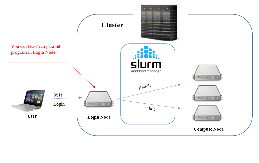
Jobs can be submitted to the cluster in several ways. Both by sending jobs to the job queue or by booking and running a node interactively.
Queueing jobs
For running time counsuming large programs, sending the job to the queue system might be preferred. You can submit a job script to the Slurm queue system from the login node with
sbatch <filename>
Warning
Note that programs should ONLY be run with sbatch above or following the instruction in Run interactively. Running programs in other way will result in the program running in the login node and not the super computer.
You can remove your job from queue with
scancel <jobid>
Information about the jobs running in the queue can be obtained with
squeue
You can also see your job in the queue by adding a flag
squeue -u <username>
The state of job is listed in the ST column. The most common job state codes are
R: Running
PD: Pending
CG: Completing
CA: Cancelled
For more job state codes please visit SLURM JOB STATE CODES.
To get further information about your jobs
scontrol show job <jobid>
These commands are the basic commands for submit, cancel, check jobs to the queue system.
Run interactively
Booking a node might be suitable if you want to test and verify your code in a parallell environment, or when the code is not time consuming but frequent adjustment is needed.
Compute nodes can be booked from the queue system for interactive use. This means that you can run your program similar to how you run it on a local computer through terminal.
Booking an interactive node can be useful when you want to test, verify or debug your code in a parallell environment. It’s also suitable when the program is not time consuming but is in need of frequent adjustment. For a large scale program we recommend Queueing jobs instead, since waiting for an interactive node booked with large amount of run time can take a lot of time.
There are two ways to book a node, using salloc and using srun.
The simplest way is to use srun command; it gives you the choice of getting
control of a node straight away (salloc will just allocate the node).
To allocate one compute node from the default partition for interactive
use just do
srun --pty bash
Depending on how busy the cluster is, it might take a while before the interactive node is booked.
Note that you can specify other options with srun, like partition, number of nodes
or if you wish to use X11 windows. For example,
srun -p cops --x11 --pty bash
will allocate a node from the cops partition and do X11 forwarding so you can use interactive programs on the compute node (like Mathematica or CST gui).
Data Management
This section gives you information about the storage solutions. Working with the HPC cluster can involve transferring data back and forth between your local machine and HPC resources. HPC offers two storage systems NFS and CFS, and an efficient usage of the requires knowing when to use what.
Where to store my data?
As the speed of CPU computations keep increasing, the relatively slow rate of input/output (I/O) or data accessing operations can create bottlenecks and cause programs to slow down significantly. Therefore it is very important to pay attention to how your programs are doing I/O and accessing data as that can have a huge impact on the run time of your jobs. Here, you will find a quick guide to storing data, ideal if you have just started to use the cluster resources.
Why is there more than one file system?
The NFS and CFS file systems offer different and often complementary functionality. The NFS is used for the home directories and CFS for the large data storage.
You can find NFS at
/cfs/homeYou can find CFS at
/cfs/nobackup
Things to remember when using all types of files:
Minimize I/O operations: larger input/output (I/O) operations are more efficient than small ones – if possible aggregate reads/writes into larger blocks.
Avoid creating too many files – post-processing a large number of files can be very hard on the file system.
Avoid creating directories with very large numbers of files – instead create directory hierarchies, which also improves interactiveness.
Running Mathematica jobs
In order to be able to use Mathematica, you have to load the program with the module load Mathematica command. The installed versions can be seen using the command module available.
Running a parallel Mathematica job involves two components:
Slurm job script
Mathematica script (the m file)
Here is a working example that finds prime numbers in parallel.
Job script job.sh
(don’t forget to change the job name when customizing the script):
#!/bin/bash -l

#SBATCH -p cops           # Partition
#SBATCH -J findprimes     # Job name
#SBATCH -N 1              # Number of nodes
#SBATCH -t 0-00:01:00     # Wall time (days-H:M:S), here = 1 hour
#SBATCH -o slurm-%j.out   # Job output file

module load Mathematica/12.1

# Optionally limit the number of launched kernels
# export MAX_CORES_LIMIT=8

math -script findprimes.m
Mathematica script findprimes.m:
<< Slurm`                       (* Load the Slurm-awareness package   *)
SlurmDebugLevel = 0;            (* Set the verbosity level (0 = none) *)
SlurmShowConfiguration[]        (* Show the used nodes and cores      *)
SlurmLaunchKernels[]            (* Launch the kernels accoringly      *)

(*****************************************************************************)
(* Parallel calculations                                                     *)
(*****************************************************************************)

Print[ "Running the main application..." ]; Print[]
primelist = ParallelTable[ Prime[k], { k, 1, 20000000 } ];
Print[ Length@primelist, "th prime is ", primelist[[-1]] ]
Print[]; Print[ "Job done!" ]

(*****************************************************************************)
(* Nice cleanup                                                              *)
(*****************************************************************************)

CloseKernels[]
Quit
Note: The package Slurm (located in
/opt/ohpc/pub/Mathematica/Applications/Slurm.m)
exposes Slurm* utility functions which can be used to launch
a number of Mathematica kernels depending on the Slurm configuration.
In the above example, we set the debug level to 0, show the Slurm configuration,
and then launch the kernels. The minimal usage consists of
<< Slurm followed by SlurmLaunchKernels[].
A Slurm job is submitted the usual way:
sbatch job.sh
After completion, the job output looks like:
Slurm configuration:

    head c03n11, cores = 64, will be used = 64

Launching Kernels...

Current wall time: 2.517 sec
Kernel count: 64

Running the main application...

20000000th prime is 373587883

Job done!
Running GPU/CUDA jobs
Note. We have one GPU node (c06n01) that is used as a toy model for testing and setting up the system. It is a NVIDIA Jetson Nano developer kit with a 128-core Maxwell GPU, Quad-core ARM A57 @ 1.43 GHz CPU, and 4 GB memory. A Supermicro server with 8x A100 Ampere cards, 2x 24-core AMD EPYC 7402 Rome @ 2.8 GHz, and 512 GB memory is expected to be installed in March 2021.
In order to be able to use CUDA, load the toolkit with the module load cuda command. There are two versions of NVIDA CUDA toolkit installed: 11.2 and 10.2. The latter version supports both x86_64 and aarch64 targets. If you wish to build a code for the aarch64 target on the x86_64 machine you also need to load Linaro cross-compiler toolchain using module load linaro-gcc.
NVIDIA Architecture
When you compile a CUDA source code, you need to specify the architecture. The supported -gencode switches are:
SM80orSM_80, compute_80for Ampere GPUs (NVIDIA A100 cards),
SM53orSM_53, compute_53for Maxwell GPUs (NVIDIA Jetson Nano Developer Kit).
The working examples can be found in Fysikum’s gitlab repository
cuda-lab-exercies,
which can be cloned with the command:
git clone https://gitlab.fysik.su.se/hpc-support/cuda-lab-exercises.git.
Below is an example how to compile and run a CUDA job for lab_1 from the repository to be run on the jetson partition, which contains Jetson Nano developer kit hardware with one 128-core Maxwell GPU.
Cross-compile the hello-world example lab01_ex1.cu for aarch64 CPU (using the -ccbin switch) with Maxwell GPU (using the -gencode switch):
ml linaro-gcc/7.3.1-2018.05
ml cuda/10.2

nvcc -O2 -m64 \
     -ccbin aarch64-linux-gnu-g++ \
     -gencode arch=compute_53,code=sm_53
     lab01_ex1.cu -o lab01_ex1
Run a test job interactively on Jetson Nano:
srun -p jetson --pty ./lab01_ex1or alternatively submit a job (here we do not need to load any CUDA module since the correct version is natively installed on the Jetson Nano GPU node):
#!/bin/bash -l

#SBATCH -p jetson
#SBATCH -N 1
#SBATCH -J cuda-L1
#SBATCH -t 01:00
#SBATCH -o test-%j.out

./lab01_ex1
Running Gaussian jobs
There are two versions of gaussian installed on the cluster:
gaussian/09.E.01-avx, which can be run on the solar and cops partitions (with or without linda)
gaussian/16.B.01-avx2, which can be run only on the cops partition (without linda).
Examples of the Slurm scripts for typical scenarios are given below. Note that g16 can also be run from the Nix environment.
g09 without linda
Script job-g09.sh:
#!/bin/bash -l

#SBATCH -p solar
#SBATCH -J g09-test-H20
#SBATCH -N 1

cat $0

ml gaussian/09.E.01-avx

g09 water9.inp
Input file example water9.inp:
%chk=water9.chk
#HF/6-31G(d,p) opt

c

0 1
1 1.0000 0.0000 0.0000
8 0.0000 0.0000 0.0000
1 0.0000 1.0000 0.0000
g09 using linda
Linda uses ssh to start workers on the compute nodes. For this purpose be sure to have your ~/.ssh/id_*.pub included in ~/.ssh/authorized_keys. Linda workers also need to be properly configured, whichis achieved by sourcing linda_slurm.sh bash script. Be sure to specify both -N and -c options in when submitting jobs so linda_slurm.sh has enough information to setup the workers.
Script job-g09-linda.sh (the example runs g09 on 4 nodes in the solar partition):
#!/bin/bash -l

#SBATCH -p solar
#SBATCH -J g09l-test-H2O
#SBATCH -N 4
#SBATCH -c 12

# Loaad the gaussian module

ml gaussian/09.E.01-avx

# Set the GAUSS environment variables based on the Slurm configuration

. linda_slurm.sh
export GAUSS_MDEF='29GB'  # %Mem Link0 definition

# Print debugging information

echo "------------"; cat $0
echo "------------"; env | grep -E "SLURM|GAUSS" | sort
echo "------------"; echo

# Run gaussian

g09 water-linda.inp
Script linda_slurm.sh:
###############################################################################
# BEGIN Slurm, set the GAUSS environment variables based on the Slurm config
###############################################################################

# GAUSS_WDEF : substitutes for %LindaWorkers, comma separated list of nodes
# GAUSS_PDEF : substitutes for %NProcShared, set by --cpus-per-task
# GAUSS_MDEF : memory per node (substitutes for %Mem)
# GAUSS_LFLAGS : options passed to the Linda proces (e.g., add -vv to debug)

export TMP_TSNET_NODES="tsnet.nodes.$SLURM_JOBID"

scontrol show hostnames "$SLURM_NODELIST" | sort -u > $TMP_TSNET_NODES

function join_by() { local IFS="$1"; shift; echo "$*"; }

export GAUSS_WDEF="$(join_by ',' $(<$TMP_TSNET_NODES))"
export GAUSS_PDEF="$SLURM_CPUS_PER_TASK"
export GAUSS_MDEF='20GB'
export GAUSS_LFLAGS="-nodefile tsnet.nodes.$SLURM_JOBID -opt 'Tsnet.Node.lindarsharg: ssh'"
# export OMP_NUM_THREADS=1

# Schedule cleanup

function rm_temp_files {
  echo; echo "Removing $TMP_TSNET_NODES"
  rm $TMP_TSNET_NODES
}

trap rm_temp_files EXIT

###############################################################################
# END Slurm
###############################################################################
Input file example water-linda.inp:
%Chk=water-linda
# RHF/6-31G(d)

water energy

0  1
O
H  1  1.0
H  1  1.0  2  120.0
g16 (as module)
Script job-g16.sh:
#!/bin/bash -l

#SBATCH -p cops
#SBATCH -J g16-test-H2O
#SBATCH -N 1

cat $0

ml gaussian/16.B.01-avx2

export PGI_FASTMATH_CPU=sandybridge

g16 water16.inp
Input file example water16.inp:
%Chk=water16.chk
# RHF/6-31G(d)

water energy

0  1
O
H  1  1.0
H  1  1.0  2  120.0
g16 (nix variant)
The gaussian g16 is also part of the NixOS-Qchem overlay, which is available on the cluster. The following script uses g16 from the Qchem overlay (note that g16 runs from the Nix environment, so be sure to have ml nix before sbatch-ing the script).
Script job-g16-nix.sh:
#!/usr/bin/env nix-shell
#!nix-shell -i bash -p gaussian

#SBATCH -p cops
#SBATCH -J g16-test-H2O
#SBATCH -N 1

cat $0

export PGI_FASTMATH_CPU=sandybridge

g16 water16.inp
Conda environments
There are currently two system-wide conda environments which are available
as modules: conda and cmbenv.
The modulefile conda comes with common
software tools like jupyter, python3 and mpi4py, while cmbenv also includes
TOAST along with all ecessary dependencies.
Below are the notes about their usage and how they can be customized.
Using Conda
To load and activate the conda software environment do the following:
module load conda
After this, jupyter and many other common software tools will be in
your environment, including a Python3 stack with mpi4py;
execute env_info to see all the software which is part of the framework.
Note that here is no need to do any ‘source’ or ‘conda activate’ command
after loading the modulefile. The lua-based module will handle this
automaticaly. Loading the module is also reversible;
use module unload conda to remove the environment.
Conda family of environments
cmbenv and conda modules are part of the same family and cannot
be loaded at the same time. Swapping these modules works perfectly
fine, for example:
module load conda
module swap conda cmbenv/0.2
module swap cmbenv/0.2 conda/0.1
Installing a personal copy of miniconda
To install your own (mini)conda environment at Sunrise, use the installation script from the following repo:
For example, to install the conda environment in ~/.local-co,
just do the following:
cd ${HOME}
git clone https://gitlab.fysik.su.se/hpc-support/conda-env.git
cd conda-env
./install-conda.sh
For the information about how to customize the installation, see README.
Using TOAST at Sunrise
A recent version of TOAST is already installed at the cluster, along with all ecessary dependencies. You can use this installation directly, or use it as the basis for your own development.
To load the software do the following:
module load cmbenv
After this, TOAST and many other common software tools will be in
your environment, including a Python3 stack; execute env_info to see
all the software which is part of the framework.
Note that here is no need to do any ‘source’ command after loading the
modulefile. The lua-based module will handle this automaticaly.
Loading the module is also reversible;
use module unload cmbenv to remove the environment.
Conda family of environments
cmbenv and conda modules are part of the same family and cannot
be loaded at the same time. Swapping these modules works perfectly
fine, for example:
module load conda
module swap conda cmbenv/0.3
module swap cmbenv conda/0.1
Installing a personal copy of TOAST
If you wish to build your own copy of TOAST and cmbenv, use the following guide with some handy installation scripts:
For example, to install the conda environment in ~/.local-so, just do
the following:
cd ${HOME}
git clone https://gitlab.fysik.su.se/hpc-support/simonsobs.git
cd simonsobs
sbatch install-all.sh
Note that the installation takes 30 minutes and consumes roughly 3.5 GiB of disk space.
For the information about how to customize the installation, see README.
Jupyter Notebook
Jupyter Notebook that employs computing intensive calculations should be run on compute nodes. The usage procedure consists of the following steps:
Login on a head node (e.g. sol-login), allocate one or more compute nodes and start jupyter.
Establish an additional ssh tunnel to the allocated compute node.
Open the link provided by Jupyter Notebook in a web browser.
Step 1. Start Jupyter Notebook.
Login via ssh to sol-login, load the conda environment
(e.g., module load conda if using the system-wide conda),
then execute:
srun --pty jupyter-notebook --no-browser --port=8889 --ip=0.0.0.0
Note that one can specify additional options when executing srun,
like the partition name using -p. These options should be placed
before --pty, e.g., srun -p cops --pty ....
Upon execution, Jupyter Notebook provides two important parameters which are needed for the next steps: (1) a name of the allocated compute node and (2) the URL with a token.
Jupyter Notebook output example
To access the notebook, open this file in a browser:
    file:///cfs/home/user/...
Or copy and paste one of these URLs:
    http://c02n01:8889/?token=6f...
 or http://127.0.0.1:8889/?token=6f...
c02n01http://127.0.0.1:8889/?token=6f....Step 2. Establish an additional ssh tunnel.
To access the compute node we need to open a new ssh connection.
This is done by specifying ssh option -NL 8889:name:8889.
Warning
This step is done on the client side in parallel to Step 1 (e.g., in a new Linux terminal or Windows WSL window).
ssh -p 31422 -NL 8889:c02n01:8889 user@sol-login.fysik.su.se
In this example we used c02n01 as the compute node.
Do not forget to replace it with a real node name that was
allocated with srun. The option -N means not to execute
any remote command (i.e., ssh creates only a tunnel and does nothing else).
Step 3. Connect to the URL.
Finally, open a browser on your client computer and copy/paste the URL with the token that was reported by Jupyter Notebook in Step 1.